Let us change our traditional attitude to the construction of programs: Instead of imagining that our main task is to instruct a computer what to do, let us concentrate rather on explaining to human beings what we want a computer to do.
Donald E. Knuth, Literate Programming (1984)
8.1 Learning objectives
By the end of this chapter the reader should be able to:
Explain the idea of literate programming from Knuth, and the reproducibility argument that Buckheit and Donoho drew from it, that the article is only advertising and the scholarship is the code and the instructions.
Trace the R lineage of literate tools from Sweave through knitr and R Markdown to Quarto, and state what each contributed.
Build a sealed render, a document whose every number and figure is regenerated from the code that produces it, and recognise the landmines that quietly break the seal.
Choose between HTML and PDF output and name the toolchain each requires, including why a LaTeX distribution belongs in the image rather than on the host.
Explain why a rendered PDF or HTML file does not hash identically across renders, and why verification therefore hashes the computational outputs rather than the rendered document.
Judge how heavily the literate-programming machinery bears on each research archetype, from the manuscript and the blog to the R package and the simulation study.
8.2 Orientation
Consider a familiar scene from a clinical-trial analysis. The statistician has a results table in the manuscript, produced months ago, and a script that, re-run today, produces a subtly different table: a mean that has moved in the third decimal, a confidence interval that no longer matches the sentence that interprets it. Neither the prose nor the code is obviously wrong. What has failed is the correspondence between them. The number in the paragraph was copied, by hand, from an analysis that has since been edited, and the paragraph was never updated. The document and its analysis have drifted apart, silently, and no one noticed until a reviewer asked how the interval was computed.
This chapter is about closing that particular gap, the gap between the prose a reader sees and the code that produced the numbers in it. The instrument is literate programming, by which we mean the practice of writing the narrative and the computation in a single source document, so that the figures and numbers a reader sees are not pasted in but regenerated every time the document is built. We shall call a document with this property a sealed render: prose bound to the code that produces every number and figure it reports, so that the document cannot silently disagree with its own analysis.
The reader will recall the ladder of reproducibility levels that organises this book: L0 locatable, L1 pinned packages, L2 pinned environment, L3 verified. It is worth stating at the outset where a sealed render sits on that ladder, because the answer is not what a newcomer expects. A sealed render is, on its own, a property almost orthogonal to the ladder. It guarantees that the document agrees with the code, but it says nothing about whether the packages are pinned, whether the environment is fixed, or whether the outputs have been verified. One can have a beautifully sealed document that runs only on its author’s laptop, at L0, and one can have a fully pinned L2 environment whose report pastes its numbers in by hand. The seal and the pins are different virtues, and much of the discipline of this chapter lies in not confusing them.
That said, the sealed render is the natural home for the machinery of the earlier chapters. It is where the pinned packages of Chapter 5 and the pinned environment of Chapter 6 are actually exercised, because it is the thing that runs the code. And it is the artifact that continuous integration renders on every change, as we shall see in Chapter 10. The sealed render is therefore the hinge between capturing an environment and validating that the capture suffices.
8.3 The analyst’s contribution
Three judgements in this chapter are the analyst’s own, and no tool makes them.
Deciding what the document computes at build time and what it merely loads. A figure regenerated on every render cannot drift from the text, which argues for computing everything in the document. A model that takes an hour to fit cannot be re-fitted on every render, which argues for computing it once in a script and caching the result. Where to draw this line, between the code that lives in the sealed document and the code that lives in analysis/scripts/ with its output saved to derived_data/, is a design decision the analyst makes for each project, and it trades the strength of the seal against the cost of the render.
Keeping the render sealed by refusing to reach outside it. A sealed render must draw only on what is captured and committed. The temptations to reach outside are many and quiet, and we catalogue them below as landmines: installing a package at render time, loading with pacman::p_load, reading a file by its absolute path on the author’s machine, depending on state left in the session by a previous chunk, reading a file that was never committed. Each produces a document that renders perfectly for its author and fails for everyone else. No linter catches all of them; the discipline is the analyst’s.
Matching the claim to what the render actually seals. A sealed render seals prose to code. It does not, by itself, seal code to its dependencies, nor dependencies to an environment, nor establish that the outputs are correct. The analyst who says ‘the analysis is reproducible’ because the report renders has claimed more than the seal delivers. The honest claim names the level actually reached, and we return to this below.
NoteThe vocabulary of this chapter
Literate programming. Writing narrative prose and executable code together in one source document, so the document is at once the program and its explanation. The term is Knuth’s.
Sealed render. A document in which every reported number and figure is regenerated from the code that produces it on each build, so the prose cannot drift from the analysis.
Code chunk. A block of executable code embedded in a literate document, delimited from the prose, whose output is inserted into the rendered document at the chunk’s position.
Render (verb and noun). To execute a literate source document and produce a finished output file (HTML, PDF, Word); and the resulting file itself.
Rendering toolchain. The programs a render invokes behind the scenes: knitr or the Quarto engine to run the code, pandoc to convert the result, and, for PDF, a LaTeX distribution to typeset it.
Determinism (of a render). The property that rendering the same source under the same environment produces a byte-for-byte identical output file. A rendered PDF is usually not deterministic in this strict sense, for reasons developed below.
SOURCE_DATE_EPOCH. A conventional environment variable, honoured by many document tools, that fixes the timestamp a build embeds, so that two builds do not differ merely because they ran at different moments.
Landmine. A pattern in a document that makes the render succeed for its author and fail for a later reader, by reaching outside the captured and committed material.
8.4 The oldest idea in the book
The idea is Knuth’s, and it is nearly as old as the practice of scientific computing itself. In 1984 Knuth proposed that a program should be written as a work of literature, a connected narrative addressed to a human reader, from which the machine-executable code is extracted mechanically (Knuth, 1984). He called the practice literate programming, and inverted the usual priority: the explanation is primary and the code is embedded within it, rather than the code being primary and the comments an afterthought. Knuth’s own motive was the comprehensibility of programs. The application to reproducible research came later, and from a different quarter.
That application, and the sentence this book takes as its keystone, is due to Buckheit and Donoho, writing in 1995 about their WaveLab software and paraphrasing their colleague Jon Claerbout (Buckheit & Donoho, 1995). Their argument, in its clearest form, is this: an article about computational science is not the scholarship itself, it is merely advertising of the scholarship; the actual scholarship is the complete software environment and the complete set of instructions that generated the figures. The claim is worth pausing over, because it reframes what a paper is. On this view the printed figures and tables are not the result but a picture of the result, and a picture can be a faithful likeness or a flattering one. The result itself, the thing that can be checked and built upon, is the code and the instructions that produce the figures. A paper that advertises a result it cannot regenerate has, in Claerbout’s sense, advertised scholarship it does not possess.
Literate programming is the technique that closes the distance between the advertisement and the scholarship. If the figure in the paper is generated, at build time, by code that lives in the same document as the prose around it, then the advertisement and the scholarship are the same artifact. The figure cannot be a flattering likeness of a result the code does not produce, because the figure is the output of the code. This is the whole of the reproducibility argument for literate programming, and every practical detail in the rest of this chapter is in service of it.
8.5 From Sweave to Quarto
The R ecosystem has realised Knuth’s idea four times over, each realisation improving on the last, and a reader will meet all four in existing code, so it is worth knowing the lineage.
The first was Sweave, introduced by Friedrich Leisch around 2002 and shipped with R itself. Sweave let an author interleave R code with LaTeX prose in a single .Rnw file, ran the code, and wove the results into a LaTeX document. It proved the concept for R and served for a decade, but it was tied to LaTeX, awkward to extend, and offered little control over how code and output were formatted.
The second, and the decisive advance, was knitr, written by Yihui Xie and released in 2012 (Xie, 2015). knitr generalised Sweave in two directions at once. It decoupled the computation from the output format, so that the same code chunks could be woven into LaTeX, into HTML, or into Markdown; and it gave the author fine control over each chunk through chunk options, the echo, eval, warning, and fig.cap settings that recur throughout this book. knitr is still the engine underneath most R literate documents, including the executable chunk later in this chapter.
The third was R Markdown, which paired knitr with pandoc, the universal document converter (Xie et al., 2018). The author now wrote in Markdown, a light and readable prose syntax, rather than in LaTeX, and pandoc converted the woven Markdown into whatever final format was wanted: HTML for the web, PDF by way of LaTeX, Word for a collaborator who redlines in track changes. This is the report.Rmd that the zzcollab templates scaffold, and the format in which a great deal of current health-sciences analysis is written.
The fourth and most recent is Quarto, released by Posit in 2022 and documented by Allaire and colleagues (Allaire et al., 2024). Quarto is best understood not as a replacement for R Markdown but as its generalisation beyond R. It keeps the knitr engine as one option, adds a Jupyter engine for Python and Julia, unifies the chunk-option syntax across languages into the #| comment form used in this book, and standardises the production of books, websites, and journal articles from the same source. This very book is a Quarto book. For an R analyst the migration from R Markdown to Quarto is small, and the two will coexist for years; the important point is that all four tools implement the same idea, and that the idea, not the tool, is what secures the seal.
NoteCheck your understanding: advertisement and scholarship
Buckheit and Donoho call the published article ‘advertising’. In one or two sentences, say what they identify as the scholarship itself, and explain how a literate document makes the advertisement and the scholarship the same object.
The scholarship is the complete software environment and the complete set of instructions that generated the figures, not the printed figures themselves. A literate document collapses the two because the figure a reader sees is produced, at build time, by the code embedded in the same document; the advertisement is therefore the output of the scholarship rather than a hand-copied picture of it, and cannot misrepresent a result the code does not produce.
8.6 The sealed render
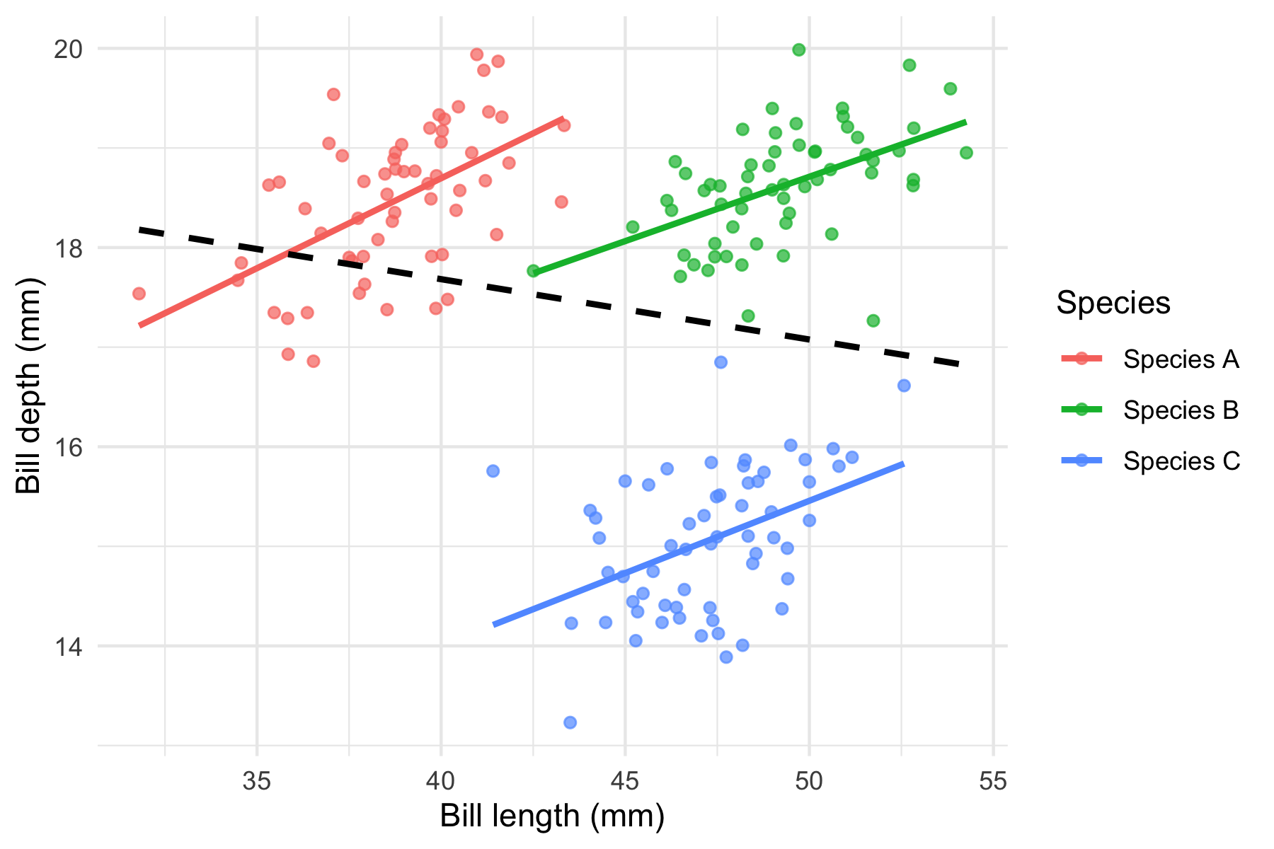
We can now make the central idea concrete, and the natural way to do so is to compute something. The following chunk generates a small synthetic dataset in the spirit of the Palmer penguins, three species measured on two bill dimensions, fits a within-species and a pooled relationship, and draws the result. The point of the exercise is not the statistics, which are a textbook instance of Simpson’s paradox, but the mechanism: this figure is produced when the book is built, from the code the reader sees, and it cannot therefore disagree with the sentences around it.
Figure 8.1: The reversal of an association upon pooling. Within each synthetic species bill depth rises with bill length (solid lines); across the pooled sample the fitted line falls (dashed). Because the figure is computed when the book is built, the described reversal cannot drift from the code that produces it.
Within each of the three synthetic species, bill depth rises with bill length: the three solid lines slope upward. Pooled across the species, the relationship reverses, and the dashed line slopes down, because across species longer bills are associated on average with shallower ones. This is Simpson’s paradox, and it is a useful thing for a figure to show. For our purposes, however, the statistical lesson is secondary. The methodological lesson is that the preceding paragraph is safe to write. If a later edit changed the synthetic means so that the pooled line no longer reversed, the figure would change on the next render and the paragraph would become visibly false, prompting its correction. In a document that pasted the figure in as a static image, the paragraph could go on asserting a reversal the data no longer showed, indefinitely. The seal is precisely this coupling: the prose and the picture rise and fall together because they are the same computation.
Two properties of the chunk are worth naming, because they are what keeps it sealed. First, it draws its data from set.seed() and rnorm(), not from a file on the author’s disk, so it carries its inputs with it. Second, it loads only packages that the build environment is known to provide, and installs nothing. A chunk that violated either property might still render on the author’s machine and would fail on anyone else’s. The next section is a catalogue of exactly these violations.
8.7 The landmines that break the seal
A sealed render is fragile in a specific way: it holds only if everything the render touches is captured and committed. Several common patterns reach outside that boundary, and each produces the same failure signature, a document that renders flawlessly for its author and errors, or worse renders differently, for a later reader. The zzcollab publishing playbook calls these landmines, and the name is apt, because they lie undetonated in a document that works until the moment someone else steps on it. We take the principal ones in turn.
The first is installing packages at render time. A chunk that calls install.packages('somepkg') or pak::pak('somepkg') during the render reaches out to a package repository as it builds, which makes the render depend on network access, on the repository’s state on the day of the render, and on whatever version is current then. The remedy is that provisioning belongs in the environment, the Dockerfile and the lockfile of the earlier chapters, never on the render path. A sealed render installs nothing; it assumes its packages are already present, pinned, and captured.
The second, a specific and common case of the first, is loading with pacman::p_load. The pacman package offers p_load(), which installs a package if it is missing and then loads it, in one call. It is convenient in interactive exploration and poisonous in a sealed render, for two compounding reasons. It installs at render time, with all the fragility just described; and it defeats static dependency discovery. Tools such as renv find a project’s dependencies by scanning the source for library(), require(), and pkg::fun() calls; they do not parse the argument list of p_load(a, b, c), so packages loaded that way go unrecorded in the lockfile and silently absent from the next machine. The remedy is to replace pacman::p_load(a, b, c) with explicit library(a), library(b), library(c) calls, which both name the dependencies for renv and load without installing.
The third is absolute host paths. A chunk that reads /Users/jsmith/data/cohort.csv, or sources a LaTeX preamble from ~/shr/preamble.tex, embeds a fact about one particular machine into the document. The path exists on the author’s laptop and nowhere else, so the render fails the moment the document moves into a container, onto a colleague’s machine, or into continuous integration. The remedy is that every file a render touches must live inside the compendium and be referenced by a relative path, so that the document carries its inputs with it.
The fourth is hidden state. A document renders its chunks in order, in a single R session, and it is easy to write a chunk that depends on an object created in an earlier chunk, or on an option set earlier, or on a package attached earlier, without saying so. The document renders correctly from top to bottom and fails when a reader runs the chunk in isolation, or when a chunk is reordered, or when caching skips the chunk that created the state. A related anti-pattern is a chunk that calls rm(list = ls()) to force a clean slate; it does not actually deliver one, since attached packages and changed options survive it, and it can delete objects the rendering harness itself relies on. The remedy is a discipline of self-contained chunks and, at the level of the toolchain, rendering each document in a fresh session so that no state leaks in from the author’s console.
The fifth is reading uncommitted files. A chunk may read a file that exists in the author’s working directory but was never committed to version control, a scratch CSV, a manually downloaded spreadsheet, an intermediate the author produced by hand. The render succeeds for the author, whose working tree contains the file, and fails for anyone who clones the repository, whose working tree does not. This is the subtlest landmine, because version control hides it: the document and the file both sit in the author’s directory, and only a clean checkout reveals that one of them was never tracked. The remedy is that a sealed render reads only committed inputs, and the surest test is to render from a fresh clone.
WarningWarning
Every landmine in this section shares one signature: the render succeeds on the author’s machine. Local success is therefore no evidence that a render is sealed. The only convincing test is a render in a clean environment that carries none of the author’s accumulated state, which is exactly what a container, or continuous integration, provides. We develop that test in Chapter 10; for now, the reader should treat ‘it renders for me’ as the beginning of the question, not the end.
NoteCheck your understanding: diagnosing a landmine
A colleague’s report.Rmd renders on her laptop but fails in continuous integration with the message ‘cannot open file: data/interim.csv’. Name two distinct landmines that could produce this symptom, and give the one-line check that would distinguish them.
The two candidates are an absolute or author-specific path, and an uncommitted file. They are distinguished by inspecting version control: if data/interim.csv is tracked and committed, the failure is more likely a path problem or a working-directory assumption; if git status or git ls-files shows the file is untracked, it is the uncommitted-file landmine, and the file must be committed (or the chunk that generates it must be included in the render) before the render can seal. Rendering from a fresh clone of the repository reproduces the CI failure locally and settles the matter.
8.8 HTML or PDF, and the toolchain each needs
A literate source document is format-agnostic; the same report.Rmd can render to HTML, to PDF, or to Word. The choice of format is not merely cosmetic, however, because each format invokes a different toolchain behind the render, and the environment must carry whatever the chosen format needs.
HTML is the lighter of the two. Rendering to HTML runs the code with knitr and converts the result with pandoc, and both are modest, self-contained dependencies. HTML is the natural default for a working analysis, for a blog post, and for anything read on a screen; it supports interactive figures, it degrades gracefully, and it imposes the smallest environmental burden. For most of a project’s life, and for every archetype whose output is read rather than submitted, HTML is the sensible target.
PDF is heavier, because a PDF is typeset, and typesetting in this ecosystem means LaTeX. Rendering to PDF runs the same knitr and pandoc steps and then hands the result to a LaTeX distribution, which lays out the pages, resolves the cross-references, sets the mathematics, and embeds the fonts. A LaTeX distribution is large, on the order of a gigabyte for a full installation, and its absence is the single most common cause of a PDF render failing on a machine where the HTML render succeeds. This is precisely the environmental problem the earlier chapters solved, and it is why the framework’s publishing profile exists. The publishing profile builds on the rocker/verse base image, which carries a LaTeX distribution baked in, so that a PDF render works inside the container with no runtime install. A project that renders to PDF chooses the publishing profile at initialisation; a project that renders only to HTML does not need it, and pays neither the build time nor the image size that the LaTeX toolchain costs. The playbook that migrates a compendium to the publishing profile turns on exactly this question: it scans every report’s YAML for a pdf_document or latex_engine output and, finding one, concludes that the verse base is required.
The general principle is the one that runs through the whole book. The literate document declares what it wants to be, and the environment must be provisioned to supply it. HTML asks little; PDF asks for LaTeX; and the honest way to supply LaTeX is to pin it in the image, not to install it, fragilely and at render time, on whatever machine happens to build the document.
8.9 Why a rendered document will not hash the same twice
We come now to a subtlety that surprises many analysts and that shapes how verification is done in Chapter 10. It is natural to suppose that the way to check a reproducible report is to render it twice and compare the two output files: if the analysis is reproducible, surely the PDFs should be identical? They will not be, and the reason is instructive.
A rendered PDF, and to a lesser degree a rendered HTML file, embeds metadata that has nothing to do with the analysis and everything to do with the moment of the render. A PDF carries a creation timestamp and a modification timestamp in its metadata; it carries an internal document identifier, often randomly generated; and when it subsets the fonts it uses, it assigns those subsets internal names that can vary between builds. Two renders of byte-for-byte identical source, in the same environment, minutes apart, therefore produce two PDF files that differ in their bytes, even though every number and figure in them is identical. The difference is real at the level of the file and spurious at the level of the science.
Part of this non-determinism can be normalised away. Many document tools, including LaTeX and pandoc, honour a conventional environment variable, SOURCE_DATE_EPOCH, which fixes the timestamp the build embeds to a specified value rather than reading the wall clock. Setting it removes the timestamp difference, and a determined practitioner can normalise further, stripping identifiers and canonicalising font-subset names, until two renders do hash alike. This is worthwhile work in some settings, notably in the reproducible-builds movement for operating systems. For a research compendium it is usually effort misplaced, because it fights the symptom rather than addressing the target.
The resolution the framework adopts is to hash the right thing. Verification, developed in Chapter 10, does not hash the rendered document. It hashes the computational outputs, the derived datasets, the model objects, the figure data, the numbers themselves, which are deterministic under a fixed environment and a fixed seed in a way the typeset PDF is not. The rendered report is a human-facing artifact, a faithful presentation of those outputs, and it is checked by regenerating it and confirming that the outputs it presents match the recorded baseline, not by demanding that its bytes be identical. It is worth noting that the framework goes further in the opposite direction for provenance: its render hook deliberately stamps each rendered PDF with the render time and the git version of the source, in a footer, precisely so that a reader can tell two renders apart and trace each to its source commit. The rendered document is thus treated as a dated, signed presentation of a result, not as the hashable object of record. The object of record is the computation.
ImportantThe honest level
A sealed render is easily mistaken for a reproducibility guarantee, and it is not one. The seal establishes that the document agrees with the code that produced it, which is level-agnostic: a sealed report can sit at L0, running only on its author’s machine. To claim L1 the packages must be pinned in a lockfile; to claim L2 the environment must be fixed in a container or a Nix declaration; to claim L3 the outputs must have been regenerated and shown to match. ‘The report renders’ is a claim about the seal, not about the level. Match the claim to the level actually reached, and state plainly that a render which succeeds on one machine has demonstrated the seal and nothing above it.
8.10 Literate programming across the archetypes
A recurring theme of this book is that a research compendium is not always a manuscript, and the weight the literate-programming machinery carries varies more across the archetypes than almost any other topic we treat. It is worth making the contrast explicit, because a reader whose mental image of a compendium is fixed on the manuscript will over-apply this chapter.
For the scholarly manuscript archetype, the sealed render is the centre of gravity. The manuscript is the product, the report.Rmd is created on the first day and grows with the analysis, and every table and figure in the eventual submission is regenerated from the code beside it. The write-as-you-go doctrine we turn to below is written for this archetype above all. Here the whole apparatus of this chapter applies at full strength.
For the blog archetype the machinery is equally central but multiplied. A blog is a collection of rendered posts rather than a single report, so the compendium renders many literate documents rather than one, and the discipline of the sealed render, no landmines, committed inputs, a pinned environment, applies to each post independently. The blog archetype stresses HTML output and the automation of rendering many documents, where the manuscript stresses PDF and the care of one.
For the data-analysis archetype the machinery is present but lighter. Such a project produces an internal report, an HTML summary for collaborators, a set of figures for a decision, rather than a typeset manuscript for submission. A sealed render is still the right way to produce that summary, and the landmines still apply, but the elaborate PDF toolchain is usually unnecessary and the document is one artifact among several rather than the organising product.
For the R-package archetype the sealed report is largely absent, and this is the sharpest contrast. An R package’s ‘document’ is not a rendered report at all; it is its help pages, generated from the roxygen comments above each function, and its vignettes, which are themselves literate documents but serve to demonstrate the package rather than to report an analysis. A package has no report.Rmd to seal because it has no single analysis to report; its literate surface is the vignette and the example, and its correctness is established by the tests and checks of Chapter 9 rather than by a rendered result. A reader building an R package should not go looking for the manuscript machinery of this chapter, because there is no manuscript.
For the simulation-study archetype the balance tips the other way again. A simulation’s output is a body of stored results, the many runs of a Monte Carlo experiment saved to derived_data/, together with a short report that summarises them. The heavy computation cannot live in the sealed document, because it takes hours or days; it lives in analysis/scripts/, is run once, seeded with care as Chapter 3 stressed, and saves its results, and the literate report then loads those results and presents them. The sealed render here is thin, a presentation layer over pre-computed results, and the reproducibility weight falls on the seeding and the storage rather than on the render. The document seals the summary to the stored results; it does not, and cannot, recompute them on each build.
The common thread is that all five archetypes share the same underlying machinery, knitr or Quarto, chunks, committed inputs, a pinned environment, and differ only in how heavily they lean on it and in what they render. The manuscript and the blog render reports and lean hard; the data analysis renders a summary and leans moderately; the package renders vignettes and help pages and leans on tests instead; the simulation renders a thin summary over stored results. One should carry the discipline of the sealed render into whichever archetype one is building, and adjust its weight to the case.
8.11 The write-as-you-go doctrine
There remains a matter of practice rather than mechanism, and it is the one on which experienced compendium authors are most insistent. The traditional order of work runs: write the analysis scripts, generate the results, then start the manuscript, and finally copy the results into the prose. This order builds the drift we opened the chapter with directly into the workflow, because the copying is manual and the results and the prose are separate artifacts from the start.
The write-as-you-go doctrine inverts the order. One creates the report.Rmd on the first day of the project, before there is any analysis to report, and writes into it the research question, the background, and the planned methods as prose. The analysis code is then added inline, in chunks, as the work proceeds, so that from the first day the numbers in the document are computed rather than copied. As patterns emerge, code that is used more than once is extracted from the document into a function in R/, and as those functions stabilise they acquire tests in inst/tinytest/, the subject of Chapter 9. When a computation grows too slow to run on every render, it moves to analysis/scripts/, is run once, and saves its result for the document to load, which is the build-time-versus-load-time boundary named among the analyst’s contributions above. The compendium’s directory structure, in this view, emerges from the writing rather than preceding it: the manuscript drives the analysis, and the R/, tests/, and scripts/ directories fill in as the code in the document matures.
The doctrine is not merely tidy. Its reproducibility payoff is that the document is sealed from the first day and stays sealed, because there is never a phase in which results live in the prose by having been copied there. The number in the paragraph was computed by the chunk above it on the very first render and on every render since, and the drift that opened this chapter has no moment at which to enter.
8.12 Worked example
Let us assemble the pieces into a concrete report.Rmd, as a health scientist beginning a cohort analysis would. On the first day, before any data are analysed, the author creates the report and writes its header. A representative YAML header, shown here as a static block rather than rendered, declares the title, the authorship, the output formats, and the bibliography:
---title:'Bill morphology across three penguin species'author:-name: A. Analystaffiliation: Department of Epidemiologydate:'July 06, 2026'output: bookdown::pdf_document2:number_sections:truekeep_tex:true bookdown::html_document2:toc:truebibliography: references.bib---
Two features of this header repay attention. The output field names two formats, a PDF built through LaTeX for submission and an HTML version for reading on a screen; the project that renders the former needs the publishing profile and its baked-in LaTeX distribution, while the latter needs neither. The date field is itself a small literate device: rather than a fixed string, it holds an inline R expression that inserts the render date, so the header cannot claim a date the render did not have. The provenance footer discussed below is not declared in this header at all; it is applied by the render tooling (make docker-render, by way of tools/stamp-render.R) rather than by the YAML.
Below the header the author writes a setup chunk that fixes the chunk defaults and loads the packages the document uses, naming each with an explicit library() call so that renv can discover them and no package is installed at render time:
From here the write-as-you-go doctrine takes over. The author writes the introduction as prose, adds a data-summary chunk, then the modelling chunk that produces the analysis, then the figure, exactly the sealed fig-simpson chunk demonstrated earlier in this chapter, which computes its result at build time and carries its synthetic inputs with it. Each number the introduction and discussion cite is inserted by an inline expression that reads the computed object, never typed by hand. Rendering the document inside the container, with make docker-render or its equivalent, executes every chunk in a fresh session, regenerates every figure, and produces the PDF and HTML, each carrying the render’s provenance footer.
The result is a document that is sealed by construction. To convince oneself that the seal holds, and does not merely appear to hold on the author’s machine, one renders it from a fresh clone of the repository inside the pinned environment. If it renders there, with no file missing and no package installed on the fly, the seal is real. If it fails, one of the landmines catalogued above has been stepped on, and the failure names which.
8.13 Collaborating with an LLM
A language model is a capable assistant for literate documents, and a treacherous one, because its fluency in producing chunks that run on the author’s machine is exactly the fluency that plants landmines. Three exchanges illustrate the pattern of use and the verification the analyst must supply.
Prompt. ‘Write a knitr chunk that loads the packages I need for this analysis and reads my cohort data.’
Watch for. A model will often reach for convenience over seal. It may emit pacman::p_load(...), or an install.packages() call, or a library(pacman) line, because these are common in the training data; and it may read the data from an absolute path it invents, such as /Users/you/data/cohort.csv, or from a path outside the project.
Verification. Insist on explicit library() calls, one per package, with no installation on the render path, and a relative path to a committed file under the compendium. Then apply the decisive test: render the chunk from a fresh clone inside the container. A chunk that survives that test is sealed; a chunk that only ran in the author’s console is not, whatever the model asserted.
Prompt. ‘My PDF render fails with a LaTeX error but the HTML render works. Fix it.’
Watch for. A model may propose to install a LaTeX package at render time, or to add a tinytex::tlmgr_install() call inside a chunk, which converts an environment problem into a render-time landmine and makes the document depend on network access and repository state.
Verification. The correct locus of the fix is the environment, not the document. Confirm that the failure is a missing LaTeX toolchain, and provision it by building on the publishing profile so that LaTeX is baked into the image, rather than installing it as the document renders. Verify that the PDF then renders in the container with nothing installed on the fly.
Prompt. ‘Check that this analysis is reproducible.’
Watch for. A model will frequently equate a successful render with reproducibility, and report the analysis as reproducible on the strength of the document having built. This conflates the seal with the level, the confusion this chapter exists to prevent.
Verification. Ask, and answer, the level question explicitly. A render that succeeds demonstrates the seal. Whether the analysis is pinned (L1), environment-fixed (L2), or verified (L3) is a separate question, settled by the lockfile, the container, and the verification command of the later chapters, not by the fact of a render. State the level actually reached and no more.
8.14 Exercises
Take an existing .Rmd or .qmd document of your own in which at least one reported number was typed into the prose by hand. Replace that number with an inline R expression that computes it from the data, render the document, and confirm the value is unchanged. Then edit the data slightly, re-render, and observe the number update in the prose. Describe what would have happened to the hand-typed number under the same edit.
Write a short knitr or Quarto chunk that generates synthetic data with set.seed() and produces a figure, as the fig-simpson chunk in this chapter does. Render it twice and confirm the figure is identical. Then remove the set.seed() call, render twice more, and explain in terms of this chapter why the figure now differs between renders and what that implies for the seal.
Deliberately plant each of the five landmines from this chapter, one at a time, in a copy of a working document: an install.packages() call, a pacman::p_load() call, an absolute host path, a chunk that depends on hidden state from an earlier chunk, and a read of an uncommitted file. For each, predict whether the document will still render on your own machine, then test the prediction by rendering from a fresh clone in a clean environment.
Locate a document in your work that renders to PDF, and determine whether the LaTeX toolchain it requires is pinned in an environment or assumed present on the host. If it is assumed present, describe the steps by which you would move it into the publishing profile, and state which reproducibility level the move would raise the project to.
Render a PDF from a literate document twice, minutes apart, and compare the two files byte for byte (for instance with a checksum). Confirm that they differ, inspect the metadata to identify what differs, and explain why hashing the rendered document would be the wrong basis for verification. Then describe what should be hashed instead.
For each of the five archetypes named in this chapter, the manuscript, the blog, the data analysis, the R package, and the simulation study, write one or two sentences stating what the literate document renders in that archetype, if anything, and how heavily the reproducibility weight rests on the render as opposed to elsewhere.
8.15 Further reading
The foundational statement of literate programming is Knuth (1984), which repays reading in the original for its inversion of the usual priority of code over explanation, even though its concrete apparatus is now of historical interest. The reproducibility argument this chapter takes as its keystone is Buckheit & Donoho (1995), whose paraphrase of Claerbout, that the article is advertising and the code and instructions are the scholarship, is the single most cited sentence in this literature and the one worth committing to memory. The earlier formulation in Claerbout & Karrenbach (1992) and the signal-processing lineage surveyed by Vandewalle et al. (2009) give the argument its original setting.
On the R realisations, Xie (2015) is the definitive treatment of knitr by its author, and Xie et al. (2018) documents R Markdown and its pandoc-based toolchain; Allaire et al. (2024) introduces Quarto and is the natural starting point for a reader beginning today. The compendium framing that binds the literate document to the rest of the project is Gentleman & Temple Lang (2007), who first proposed the compendium as an executable document, and Marwick et al. (2018), whose rrtools operationalises it around a report.Rmd. For the practical habits, Sandve et al. (2013) and Wilson et al. (2017) both stress recording exactly how each figure was produced, which is the sealed render stated as a rule of conduct. The determinism questions touched on here connect to the verification machinery of Chapter 10 and, in the wider setting of reproducible builds, to a substantial body of systems literature that a reader pursuing byte-level reproduction of documents will want to consult beyond the scope of this book.
Allaire, J. J., Teague, C., Scheidegger, C., Xie, Y., & Dervieux, C. (2024). Quarto: An open-source scientific and technical publishing system. https://quarto.org/
Claerbout, J. F., & Karrenbach, M. (1992). Electronic documents give reproducible research a new meaning. SEG Technical Program Expanded Abstracts 1992, 601–604. https://doi.org/10.1190/1.1822162
Gentleman, R., & Temple Lang, D. (2007). Statistical analyses and reproducible research. Journal of Computational and Graphical Statistics, 16(1), 1–23. https://doi.org/10.1198/106186007X178663
Marwick, B., Boettiger, C., & Mullen, L. (2018). Packaging data analytical work reproducibly using R (and friends). The American Statistician, 72(1), 80–88. https://doi.org/10.1080/00031305.2017.1375986
Sandve, G. K., Nekrutenko, A., Taylor, J., & Hovig, E. (2013). Ten simple rules for reproducible computational research. PLOS Computational Biology, 9(10), e1003285. https://doi.org/10.1371/journal.pcbi.1003285
Vandewalle, P., Kovacevic, J., & Vetterli, M. (2009). Reproducible research in signal processing. IEEE Signal Processing Magazine, 26(3), 37–47. https://doi.org/10.1109/MSP.2009.932122
Wilson, G., Bryan, J., Cranston, K., Kitzes, J., Nederbragt, L., & Teal, T. K. (2017). Good enough practices in scientific computing. PLOS Computational Biology, 13(6), e1005510. https://doi.org/10.1371/journal.pcbi.1005510
Xie, Y. (2015). Dynamic documents with R and knitr (2nd ed.). Chapman; Hall/CRC.